2. Add Two Numbers

题目描述

给出两个 非空 的链表( linked lists)用来表示两个非负的整数。其中，它们各自的位数是按照 逆序 的方式存储的，并且它们的每个节点只能存储 一位 数字。

如果，我们将这两个数相加起来，则会返回一个新的链表来表示它们的和。

您可以假设除了数字 0 之外，这两个数都不会以 0 开头。

示例

1
2
3

输入：(2 -> 4 -> 3) + (5 -> 6 -> 4)
输出：7 -> 0 -> 8
原因：342 + 465 = 807

Solution

1
2
3
4
5
6
7
8
9
10
11
12
13
14
15
16
17
18
19
20
21
22
23
24
25
26
27
28
29
30
31

# Definition for singly-linked list.
class ListNode:
    def __init__(self, x):
         self.val = x
         self.next = None

class Solution:
    def addTwoNumbers(self, l1, l2):
    # def addTwoNumbers(self, l1: ListNode, l2: ListNode) -> ListNode:
        """
        :type l1: ListNode
        :type l2: ListNode
        :rtype: ListNode
        """
        head = curr = ListNode(0)
        carry = 0 # 进位
        while l1 or l2:
            # 从低到高 逐位相加
            sum = carry
            if l1:
                sum += l1.val
                l1 = l1.next
            if l2:
                sum += l2.val
                l2 = l2.next
            curr.next = ListNode(sum%10)  # 个位保留 十位做进位
            curr = curr.next
            carry = sum / 10
        if carry > 0: # 特别注意 两个链表都加完后是否还有进位
            curr.next = ListNode(carry)
        return head.next

注意

1.Python2用/ Python3用 // 表示下取整的除法
2.链表的构建

1
2
3
4
5
6

head = curr = ListNode(0)
...
curr.next = ListNode(XX)
curr = curr.next
...
return head.next

3.生成链表的方法及本题测试代码

1
2
3
4
5
6
7
8
9
10
11
12
13
14
15
16
17
18
19
20
21
22
23

def generateList(l: list) -> ListNode:
    prenode = ListNode(0)
    lastnode = prenode
    for val in l:
        lastnode.next = ListNode(val)
        lastnode = lastnode.next
    return prenode.next


def printList(l: ListNode):
    while l:
        print("%d, " %(l.val), end = '')
        l = l.next
    print('')

if __name__ == "__main__":
    l1 = generateList([1, 5, 8])
    l2 = generateList([9, 1, 2, 9])
    printList(l1)
    printList(l2)
    s = Solution()
    sum = s.addTwoNumbers(l1, l2)
    printList(sum)

3. Longest Substring Without Repeating Characters

题目描述

给定一个字符串，请你找出其中不含有重复字符的 最长子串 的长度。。

示例

1
2
3
4
5
6
7
8
9
10
11
12

输入: "abcabcbb"
输出: 3 
解释: 因为无重复字符的最长子串是 "abc"，所以其长度为 3。

输入: "bbbbb"
输出: 1
解释: 因为无重复字符的最长子串是 "b"，所以其长度为 1。

输入: "pwwkew"
输出: 3
解释: 因为无重复字符的最长子串是 "wke"，所以其长度为 3。
     请注意，你的答案必须是 子串 的长度，"pwke" 是一个子序列，不是子串。

Solution1

1
2
3
4
5
6
7
8
9
10
11
12
13

class Solution:
    def lengthOfLongestSubstring(self, s: str) -> int:
        max_len = 0 # 储存最大长度
        start = 0 # 记录子串开始的index
        substring = {}
        for index, c in enumerate(s):
            # 不断记录下子串，直到出现重复字符，记录下原子串的长度，
            # 并丢弃原子串中该字符及之前的字符（更新start位置），将新的字符加入子串中
            if c in substring and substring[c] >= start:
                max_len = max(max_len, index-start)
                start = substring[c] + 1
            substring[c] = index
        return max(max_len, len(s) - start)  #遍历到最后的一串无重复字符子串长度为len(s)-start

Solution2

1
2
3
4
5
6
7
8
9
10
11
12
13

class Solution:
    def lengthOfLongestSubstring(self, s: str) -> int:
        substring = ""
        max_len = 0
        for c in s:  
            index = substring.find(c)  # 直接对字符串操作
            if index == -1:
                substring += c
            else:
                max_len = max(max_len, len(substring))         
                substring = substring[index+1:] + c  #注意这里不是[index+1:-1]
            
        return max(max_len, len(substring))

5. Longest Palindromic(回文) Substring ！！！！！！！！！！！！！！！！

题目描述

给定一个字符串 s，找到 s 中最长的回文子串。你可以假设 s 的最大长度为 1000。

示例

1
2
3
4
5
6

输入: "babad"
输出: "bab"
注意: "aba" 也是一个有效答案。

输入: "cbbd"
输出: "bb"

Solution

6. ZigZag Conversion (Z字形变换)

相关标签: 字符串

题目描述

将一个给定字符串根据给定的行数，以从上往下、从左到右进行 Z 字形排列。

比如输入字符串为 “LEETCODEISHIRING” 行数为 3 时，排列如下：

1
2
3

L   C   I   R
E T O E S I I G
E   D   H   N

之后，你的输出需要从左往右逐行读取，产生出一个新的字符串，比如：”LCIRETOESIIGEDHN”。

请你实现这个将字符串进行指定行数变换的函数 string convert(string s, int numRows);

示例

1
2
3
4
5
6
7
8
9
10
11

输入: s = "LEETCODEISHIRING", numRows = 3
输出: "LCIRETOESIIGEDHN"

输入: s = "LEETCODEISHIRING", numRows = 4
输出: "LDREOEIIECIHNTSG"
解释:

L     D     R
E   O E   I I
E C   I H   N
T     S     G

Solution

1
2
3
4
5
6
7
8
9
10
11
12
13

class Solution:
    def convert(self, s: str, numRows: int) -> str:
        if numRows < 2:
            return s
        row = ["" for _ in range(numRows)]
        row_id = 0
        flag = -1
        for c in s:
            row[row_id] += c
            if row_id==0 or row_id == numRows - 1:
                flag = -flag
            row_id += flag
        return "".join(row)

11. Container With Most Water

相关标签: 双指针

题目描述

给定 n 个非负整数 a1，a2，…，an，每个数代表坐标中的一个点 (i, ai) 。在坐标内画 n 条垂直线，垂直线 i 的两个端点分别为 (i, ai) 和 (i, 0)。找出其中的两条线，使得它们与 x 轴共同构成的容器可以容纳最多的水

示例

1
2

输入: [1,8,6,2,5,4,8,3,7]
输出: 49

Solution

1
2
3
4
5
6
7
8
9
10
11
12
13

class Solution:
    def maxArea(self, height: List[int]) -> int:
        i = 0
        j = len(height) - 1
        res = 0
        while i < j:
            if height[i] < height[j]:
                res = max(res, height[i] * (j - i))
                i += 1
            else:
                res = max(res, height[j] * (j - i))
                j -= 1
        return res

思路

算法流程： 设置双指针 i,j 分别位于容器壁两端，根据规则移动指针（后续说明），并且更新面积最大值 res，直到 i == j 时返回 res。

指针移动规则与证明： 每次选定围成水槽两板高度 h[i],h[j]中的短板，向中间收窄 111 格。以下证明：

• 设每一状态下水槽面积为 S(i,j),(0<=i<j<n)，由于水槽的实际高度由两板中的短板决定，则可得面积公式 S(i,j)=min(h[i],h[j])×(j−i)S(i, j)。
• 在每一个状态下，无论长板或短板收窄 1格，都会导致水槽 底边宽度 −1。
• 若向内移动短板，水槽的短板 min(h[i],h[j])可能变大，因此水槽面积 S(i,j)S(i, j)S(i,j) 可能增大。
• 若向内移动长板，水槽的短板 min(h[i],h[j])不变或变小，下个水槽的面积一定小于当前水槽面积。

12. Integer to Roman

相关标签: 字符串

题目描述

罗马数字包含以下七种字符： I， V， X， L，C，D 和 M。

1
2
3
4
5
6
7
8

字符          数值
I             1
V             5
X             10
L             50
C             100
D             500
M             1000

例如， 罗马数字 2 写做 II ，即为两个并列的 I。12 写做 XII ，即为 X + II 。 27 写做 XXVII, 即为 XX + V + II 。

通常情况下，罗马数字中小的数字在大的数字的右边。但也存在特例，例如 4 不写做 IIII，而是 IV。数字 1 在数字 5 的左边，所表示的数等于大数 5 减小数 1 得到的数值 4 。同样地，数字 9 表示为 IX。这个特殊的规则只适用于以下六种情况：

I 可以放在 V (5) 和 X (10) 的左边，来表示 4 和 9。
X 可以放在 L (50) 和 C (100) 的左边，来表示 40 和 90。 
C 可以放在 D (500) 和 M (1000) 的左边，来表示 400 和 900。

给定一个整数，将其转为罗马数字。输入确保在 1 到 3999 的范围内。

示例

1
2
3
4
5
6
7
8
9
10
11
12
13
14

输入: 3
输出: "III"

输入: 4
输出: "IV"

输入: 9
输出: "IX"

输入: 58
输出: "LVIII"

输入: 1994
输出: "MCMXCIV"

Solution

1
2
3
4
5
6
7
8
9
10
11
12
13
14
15
16
17
18

class Solution:
    def intToRoman(self, num: int) -> str:
        res = ""
        values = [1000, 900, 500, 400,
                  100, 90, 50, 40,
                  10, 9, 5, 4,
                  1]
        symbols = ['M', 'CM', 'D', 'CD',
                   'C', 'XC', 'L', 'XL',
                   'X', 'IX', 'V', 'IV',
                   'I']
        i = 0
        while num > 0:
            count = num // values[i]
            res += "".join([symbols[i] for _ in range(count)])
            num -= count * values[i]
            i += 1
        return res

15. 3SUM

相关标签: 双指针 数组

题目描述

给定一个包含 n 个整数的数组 nums，判断 nums 中是否存在三个元素 a，b，c ，使得 a + b + c = 0 ？找出所有满足条件且不重复的三元组。

注意：答案中不可以包含重复的三元组。

示例

1
2
3
4
5
6
7

给定数组 nums = [-1, 0, 1, 2, -1, -4]，

满足要求的三元组集合为：
[
  [-1, 0, 1],
  [-1, -1, 2]
]

Solution

1
2
3
4
5
6
7
8
9
10
11
12
13
14
15
16
17
18
19
20
21
22
23
24
25

class Solution:
    def threeSum(self, nums: List[int]) -> List[List[int]]:
        nums.sort()
        res = []
        for k in range(len(nums)-2):
            if nums[k] > 0: break
            if k > 0 and nums[k] == nums[k-1]: continue
            i, j = k+1, len(nums)-1

            while i < j:
                s = nums[k] + nums[i] + nums[j]

                if s > 0:
                    j -= 1
                    while i < j and nums[j] == nums[j+1]: j -= 1
                elif s < 0:
                    i += 1
                    while i < j and nums[i] == nums[i-1]: i += 1
                else:
                    res.append([nums[k], nums[i], nums[j]])
                    i += 1
                    j -= 1
                    while i < j and nums[j] == nums[j+1]: j -= 1
                    while i < j and nums[i] == nums[i-1]: i += 1
        return res

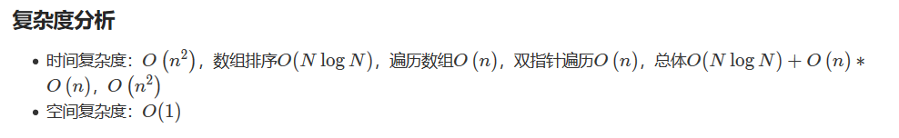
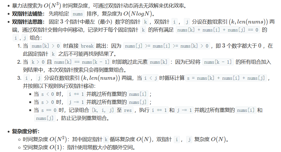
思路

16. 3Sum Closest

相关标签: 双指针 数组

题目描述

给定一个包括 n 个整数的数组 nums 和 一个目标值 target。找出 nums 中的三个整数，使得它们的和与 target 最接近。返回这三个数的和。假定每组输入只存在唯一答案。

示例

1
2
3

给定数组 nums = [-1，2，1，-4], 和 target = 1.

与 target 最接近的三个数的和为 2. (-1 + 2 + 1 = 2).

Solution

1
2
3
4
5
6
7
8
9
10
11
12
13
14
15
16
17
18
19
20
21
22
23

class Solution:
    def threeSumClosest(self, nums: List[int], target: int) -> int:
        nums.sort()
        res = float("inf")
        for k in range(len(nums)-2):
            if k > 0 and nums[k] == nums[k-1]: continue
            i, j = k+1, len(nums)-1

            while i < j:
                s = nums[k] + nums[i] + nums[j]
                if s == target:
                    return s
                elif abs(s-target) < abs(res-target):
                    res = s
                
                if s < target:
                    i+=1
                    while i < j and nums[i] == nums[i-1]: i += 1
                elif s > target:
                    j -= 1
                    while i < j and nums[j] == nums[j+1]: j -= 1
                
        return res

经验分享

本科生晋升GM记录 & Kaggle比赛进阶技巧分享

Tricks

调参技巧

1.Adam: init_lr=5e-4(3e-4)（⭐⭐⭐⭐⭐），3e-4号称是Adam最好的初始学习率

2.lr schedule

• ReduceLROnPlateau，patience=4（5），gamma=0.1，这是我常用的一套组合，并不是最好的；
• StepLR，个人比较喜欢用这个，自己设定好在哪个epoch进行学习率的衰减，个人比较喜欢用的衰减步骤是[5e-4(3e-4), 1e-4, 1e-5, 1e-6]，至于衰减位置，就需要自己有比较好的直觉，或者就是看log调参，对着2.1上训练的valid loss走势，valid loss不收敛了，咱就立刻进行衰减；
• CosineAnnealingLR+Multi cycle,这个相较于前两个，就不需要太多的调参，可以训练多个cycle，模型可以找到更多的局部最优，一般推荐min_lr=1e-6，至于每个cycle多少epoch这个就说不准了，不同数据不太一样。

3.finetune，微调也是有许多比较fancy的技巧，在这里不做优劣比较，针对分类任务说明。

• 微调方式一，最常用，只替换掉最后一层fc layer，改成本任务里训练集的类别数目，然后不做其余特殊处理，直接开始训练；
• 微调方式二，在微调一的基础上，freeze backbone的参数，只更新（预训练）新的fc layer的参数（更新的参数量少，训练更快）到收敛为止，之后再放开所有层的参数，再一起训练；
• 微调方式三，在微调方式二预训练fc layer之后或者直接就是微调方式一，可选择接上差分学习率（discriminative learning rates）即更新backbone参数和新fc layer的参数所使用的学习率是不一致的，一般可选择差异10倍，理由是backbone的参数是基于imagenet训练的，参数足够优秀同时泛化性也会更好，所以是希望得到微调即可，不需要太大的变化。

1

optimizer = torch.optim.Adam([{'params': model.backbone.parameters(), 'lr': 3e-5}, {'params': model.fc.parameters(), 'lr': 3e-4}, ])

• 微调方式四，freeze浅层，训练深层（如可以不更新resnet前两个resnet block的参数，只更新其余的参数，一样是为了增强泛化，减少过拟合）。

4.Find the best init_lr，前面说到3e-4在Adam是较优的init_lr，那么如何寻找最好的init_lr？

• 出自fastai, lr_find()，其原理就是选取loss function仍在明显降低的较大的学习速率，优劣性其实也是相对而言，不一定都是最好的。

5.learing rate warmup，理论解释可以参 https://www.zhihu.com/question/338066667

6.如果模型太大的同时你的GPU显存又不够大，那么设置的batch size就会太小，如何在有限的资源里提升多一点？

• 梯度累计（gradient accumulation），其实就是积累多个batch的梯度之后，再进行梯度的回传做参数的更新，变相的增大了训练的batch size，但缺点是对Batch Normalization没影响的。。
• 如果你卡多，这时可以使用多卡并行训练，但要使用syncbn（跨卡同步bn），即增大了batch size，又对Batch Normalization起到相同的作用。

分类赛技巧

1.label smoothing

分类任务的标签是one-hot形式，交叉熵会不断地去拟合这个真实概率，在数据不够充足的情况下拟合one-hot容易形成过拟合，因为one-hot会鼓励正确类别与所属类别之间的差异性尽可能大，但其实有不少类别之间是极为相似的。label smoothing的做法其实就是将hard label变成soft label。

2.topk-loss(OHEM)

OHEM最初是在目标检测上提出来的，但其实思想是所有领域任务都通用的。意思就是提取当前batch里top k大的loss的均值作为当前batch的loss，进行梯度的计算和回传。其insight也很简单，就是一种hard mining的方法，一个batch里会有easy sample和hard sample，easy sample对网络的更新作用较小（loss值小，梯度也会小），而hard sample的作用会更大（loss值大，梯度值也会大），所以topk-loss就是提取hard sample。

1
2
3

loss = criterion(logits, truth)
loss,_ = loss.topk(k=..)     
loss = loss.mean()

3.weighted loss

weighted loss其实也算是一种hard mining的方法，只不过这种是人为地认为哪种类别样本更加hard，哪种类别样本更加easy。也就是说人为对不同类别的loss进行进行一个权重的设置，比如0,1类更难，设置权重为1.2，2类更容易，设置权重为0.8。。

1
2
3

weights = [1.2, 1.2, 0.8]
class_weights = torch.FloatTensor(weights).to(device)
criterion = torch.nn.CrossEntropyLoss(weight=class_weights)

4.dual pooling

这种是在模型层进行改造的一种小trick了，常见的做法：global max/average pooling + fc layer，这里试concat(global max-pooling, global average pooling) + fc layer，其实就是为了丰富特征层，max pooling更加关注重要的局部特征，而average pooling试更加关注全局的特征。不一定有效，我试过不少次，有效的次数比较少，但不少人喜欢这样用。

1
2
3
4
5
6
7
8
9
10
11
12
13
14
15
16
17
18
19
20
21
22
23
24
25
26
27
28
29
30
31
32

class res18(nn.Module):
    def __init__(self, num_classes):
        super(res18, self).__init__()
        self.base = resnet18(pretrained=True)
        self.feature = nn.Sequential(
            self.base.conv1,
            self.base.bn1,
            self.base.relu,
            self.base.maxpool,
            self.base.layer1,
            self.base.layer2,
            self.base.layer3,
            self.base.layer4
        )
        self.avg_pool = nn.AdaptiveAvgPool2d(1)
        self.max_pool = nn.AdaptiveMaxPool2d(1)
        self.reduce_layer = nn.Conv2d(1024, 512, 1)
        self.fc  = nn.Sequential(
            nn.Dropout(0.5),
            nn.Linear(512, num_classes)
            )
    def forward(self, x):
        bs = x.shape[0]
        x = self.feature(x)
        x1 = self.avg_pool(x).view(bs, -1)
        x2 = self.max_pool(x).view(bs, -1)
        x1 = self.avg_pool(x)
        x2 = self.max_pool(x)
        x = torch.cat([x1, x2], dim=1)
        x = self.reduce_layer(x).view(bs, -1)
        logits = self.fc(x)
        return logits

5.margin-based softmax

• 在人脸识别领域，基于margin的softmax loss其实就是对softmax loss的一系列魔改（large margin softmax、NormFace、AM-softmax、CosFace、ArcFace等等），增加类间 margin，当然也有其它的特点，如weight norm和基于余弦角度的优化等等。其共同目标都是为了获得一个更加具有区分度的feature，不易过拟合。
• 一个比较多同学忽略的点是，如果使用了margin-based softmax，往往连同开源repo里默认的超参数也一起使用了，比如s=32.0，m=0.5，但其实这两个参数的设定都是有一定的缘由，比如s值象征着超球体的体积，如果类别数较多，那么s应该设置大点。如果你没有很好的直觉，那grid search一波，搜索到适合的s和m值也不会花很多时间。

6.Lovasz loss

• 这个loss本来是出于分割任务上的，其优化的是IOU，但你如果仔细观察lovasz传入的logit和truth，可以发现是和multi label classification类似，logit和truth都是由多个1值的one-hot形式。所以在多标签分类任务上，其实是可以用lovasz loss来进行优化的，出自（Bestfitting）(https://www.kaggle.com/c/human-protein-atlas-image-classification/discussion/78109#latest-676029)

分类赛技巧（openset/检索）

1.BNNeck(出自罗浩博士的Bag of Tricks and A Strong Baseline for Deep Person Re-identification )，知乎链接一个更加强力的ReID Baseline， 其实就是在feature层和fc layer之间增加一层Batch Normalization layer，然后在retrieval的时候，使用BN后的feature再做一个l2 norm，也就是retrieval with Cosine distance。

1
2
3
4
5
6
7
8
9
10
11
12
13
14
15
16
17
18
19
20
21
22
23
24
25
26

class res50(torch.nn.Module):
    def __init__(self, num_classes):
        super(res50, self).__init__()
        resnet = resnet50(pretrained=True)
        self.backbone = torch.nn.Sequential(
                        resnet.conv1,
                        resnet.bn1,
                        resnet.relu,
                        resnet.layer1,
                        resnet.layer2,
                        resnet.layer3,
                        resnet.layer4
        )
        self.pool = torch.nn.AdaptiveMaxPool2d(1)
        self.bnneck = nn.BatchNorm1d(2048)
        self.bnneck.bias.requires_grad_(False)  # no shift
        self.classifier = nn.Linear(2048, num_classes, bias=False)
    def forward(self, x):
        x = self.backbone(x)
        x = self.pool(x)
        feat = x.view(x.shape[0], -1)
        feat = self.bnneck(feat)
        if not self.training:
            return nn.functional.normalize(feat, dim=1, p=2)
        x = self.classifier(feat)
        return x

2.margin-based softmax（上面已经说到）

3.triplet loss + softmax loss，结合metric learning，对feature进行多个loss的优化，triplet loss也是可以有很多的花样，Batch Hard Triplet Loss，是针对triplet loss的一种hard mining方法。

4.IBN，切换带有IBN block的backbone，搜图（open-set）往往test和train是不同场景下的数据，IBN block当初提出是为了提高针对不同场景下的模型泛化性能，提升跨域（cross domain）能力，在reid下的实验，IBN表现优异。

5.center loss

6.Gem，generalized mean pooling，出自Fine-tuning CNN Image Retrieval with No Human Annotation，提出的是一种可学习的pooling layer，可提高检索性能，代码出自 https://github.com/tuananh1007/CNN-Image-Retrieval-in-PyTorch/blob/master/cirtorch/layers/pooling.py

1
2
3
4
5
6
7
8
9

class GeM(nn.Module):
    def __init__(self, p=3, eps=1e-6):
        super(GeM,self).__init__()
        self.p = Parameter(torch.ones(1)*p)
        self.eps = eps
    def forward(self, x):
        return LF.gem(x, p=self.p, eps=self.eps)
    def __repr__(self):
        return self.__class__.__name__ + '(' + 'p=' + '{:.4f}'.format(self.p.data.tolist()[0]) + ', ' + 'eps=' + str(self.eps) + ')'

7.global feature + local features 将全局特征和多个局部特征一起融合，其实就是一种暴力融合特征的方法，对提升精度有一定的帮助，就是耗时相对只使用global feature来说很多点，此种方法可参考在reid常用的PCB(Beyond Part Models: Person Retrieval with Refined Part Pooling)或MGN(Learning Discriminative Features with Multiple Granularities for Person Re-Identification)方法

8.re-ranking，是一种在首次获取检索图的候选图里做一次重新排序，获得更加精准的检索，相对比较耗时间，不适合现实场景，适合比赛刷精度。

分割赛技巧

1.Unet Unet可以说是在kaggle的语义分割赛里的一个较优的选择，许多top solution都是使用了Unet，FPN也是一个非常不错的选择。
2.Unet的魔改
现在有个开源库其实是已经集成了许多不同分割网络，表现也是相对不错的，如果觉得自己修改比较困难，或者自己改得不够好，可以尝试使用这个库segmentation_models_pytorch

• 很多top solution都是修改Unet的Decoder，最常见的就是增加scse block和Hypercolumn block，也有一些是使用了CBAM（Convolutional Block Attention Module，bestfitting比较喜欢用）或BAM（Bottleneck attention module），这些注意力block一般是放在decoder不同stage出来的feature后面，因为注意力机制往往都是来优化feature的。
• dual head(multi task learning)，也就是构造一个end2end带有分割与分类的模型。同时，多任务学习往往会降低模型过拟合的程度，并可以提升模型的性能。

1
2
3
4
5
6
7
8
9
10
11
12
13
14
15
16

import segmentation_models_pytorch as smp
class Res34_UNET(nn.Module):
    def __init__(self, num_classes):
        super(Res34_UNET, self).__init__()
        self.model = smp.Unet(encoder_name='resnet34', encoder_weights='imagenet', classes=num_classes, activation=None)
        self.avgpool = nn.AdaptiveAvgPool2d((1,1))
        self.cls_head = nn.Linear(512, num_classes, bias=False)

    def forward(self, x):
        global_features = self.model.encoder(x)
        cls_feature = global_features[0]
        cls_feature = self.avgpool(cls_feature)
        cls_feature = cls_feature.view(cls_feature.size(0), -1)
        cls_feature = self.cls_head(cls_feature)
        seg_feature = self.model.decoder(global_features)
        return seg_feature, cls_feature

3.lovasz loss 之前在TGS Salt Identification的适合，lovasz对分割的效果的表现真的是出类拔萃，相比bce或者dice等loss可以提高一个档次。但是最近的分割赛这个loss的表现就一般，猜测是优化不同metric，然后不同loss就会带来不同的效果，又或者是数据的问题。

4.dice loss for postive，bce loss for negtive 主要就是将分割任务划分两个任务：1. 分割任务，2. 分类任务 dice loss可以很好的优化模型的dice score，而bce loss训练出来的分类器可以很好地找出negtive sample，两者结合可以达到一种非常好效果，详细解说可以参考我之前的一个solution: Kaggle Understanding Clouds 7th place总结

通用技巧

1.TTA（Test Time Augmentation） 一种暴力测试的方法，将有效的增强方式得到多个不同的input，然后进行infer，得到多个结果进行融合，一般会比原始input会高不少。这种方法的缘由就是希望通过对input进行不同的变换方式获取多个不同的但重要的特征，然后可以得到多个具有差异性的预测结果。
2.多尺度训练，融合 在训练期间，随机输入多种尺度的图像进行训练，如（128128，196196，224224，256256，384*384等等）然后测试的时候可适当的选取其中某几个尺度表现优异的预测结果出来融合，这种方法其实就是为了提升模型对尺度的变换的鲁棒性，不易受尺度变换的影响。
3.Ensemble

• Snapshot Ensembles，这个方法常在与cycle learning rate的情况下使用，在不同cycle下，模型会产出多个不同的snapshot weight（多个不同的局部最优，具有差异性），这时可以将这几个snapshot model一起进行推断，然后将预测结果进行平均融合。
• SWA, Stochastic Weight Averaging，随机权重平均，其实现原理当模型在训练时收敛到一定程度后，开始追踪每次epoch后得到的模型的平均值，有一个计算公式和当前的模型权重做一个平均得到一个最终的权重，提高泛化性能。
• stacking，在分类任务里，stacking是作为一种2nd level的ensemble方法，将多个“准而不同”的基分类器的预测集成与一身，再扔进去一个简单的分类器（mlp、logit regression、simple cnn，xgboost等）让其自己学习怎么将多个模型融合的收益做到最高。一般数据没有问题的话，stacking会更加稳定，不易过拟合，融合的收益也会更高。

4.设计metric loss 许多小伙伴会有这样一个疑惑，比赛的评测metric往往和自己训练时所使用的loss优化方向不是那么一致。比如多标签分类里的metric是fbeta_score，但训练时是用了bce loss，经常可以看到val loss再收敛后会有一个反弹增大的过程，但此时val fbeta_score是还在继续提升的。这时就可以针对metric来自行设计loss，比如fbeta loss就有。

5.semi-supervised learning

• recurssive pseudo-label（伪标签），伪标签现在已经是kaggle赛里一个必备工具了，但是这是个非常危险的操作，如果没有筛选好的伪标签出来，容易造成模型过拟合伪标签里的许多噪声。比较安全的方法是：1. 筛选预测置信度高的样本作为伪标签，如分类里，再test里的预测概率是大于0.9的，则视为正确的预测，此时将其作为伪标签来使用。2. 帮第一次的伪标签扔进去训练集一起训练后，得到新的模型，按相同的规则再次挑一次伪标签出来。3. 如此不断循环多次，置信度的阈值可以适当作调整。
• mean teacher，在这里给涛哥在Recursion Cellular Image Classification第三名的方案做个广告，end2end semi-supervised learining pipeline。

• knowledge distillation（知识蒸馏），此方法有助于提高小模型（student）的性能，将大模型（teacher）的预测作为soft label（用于学习teacher的模型信息）与truth（hard label）扔进去给小模型一起学习，当然两个不同label的loss权重需要调一调。当然，蒸馏的方法有很多种，这只是其中一种最简单的方法。蒸馏不一定用于训练小模型，大模型之间也是可以一同使用的

数据增强与预处理

1.h/v flip(水平垂直翻转)，95%的情况下都是有效的，因为不怎么破坏图像空间信息。
2.random crop/center crop and resize，在原图进行crop之后再resize到指定的尺度。模型的感受野有限，有时会看不到图像中一些分布比较边缘或者是面积比较小的目标物体，crop过后其占比有更大，模型看到的机会也会更多。适用性也是比较大的。
3.random cutout/erasing(随机擦除)，其实就是为了随机擦除图像中局部特征，模型根据有限的特征也可以判断出其属性，可提高模型的泛化性。
4.AutoAugment，自己设定一些规则policy，让模型自己寻找合适的数据增强方式，需要消耗比较多的计算资源。
5.mixup 一种与数据无关的数据增强方式，即特征之间的线性插值应导致相关标签之间的线性插值，扩大训练分布。意思是两个不同的label的样本进行不同比例的线性插值融合，那么其label也应该是相同比例关系进行线性融合。（上图）
6.Class balance 主要就是针对数据不平衡的情况下进行的操作，一般是针对采样方法，或者在loss上做处理，如focal loss、weighted loss等。
7.图像预处理，许多看似有效的预处理操作，但是并不一定有效，如在医学领域的图像，许多肉眼观察良好的预处理的方式，实际上是破坏了原图真实类别关联的特征，这种方面需要相关领域知识。

如何选择更好的backbone模型

1.对于baseline，从resnet18/34 or efficientnet-B0起步，把所有work的技巧（loss/augmentation/metric/lr_schedule）调好之后，这时就应该大模型（deeper）；
2.当更好需要换模型的时候，是不是就需要自己去设计/构造新模型呢？其实在比赛的短期里，重新设计一个新的backbone出来是不提倡的，因为模型不仅要work，还要重新在imagenet上预训练，时间消耗巨大，不合适比赛；
3.由于学术界里，sota模型多之又多，那如何选择？从个人经验总结来看，比较推荐se-resnext50/101、SENet154（太大，很少用），带有se block的resnet，都不同类型的任务都有一定的通用性，性价比也较高；efficientnet系列（最近在某些比赛里还优于se-resnext）可以上到B3,B5，有条件的B7都没问题。其他的sota模型，可以尝试Xception，inception-resnetV2等等。

Competitions

0.安装

0.1 安装Anaconda3:

https://blog.csdn.net/u012318074/article/details/77074665
现在最新的版本所带的python版本应该是3.7 （找个3.6版本的也可以）

0.2 安装Pytorch

在命令行输入which pip， 应该会显示pip在anaconda3下面，这时如果用pip命令装pytorch就是装在Anaconda3里面了。

在命令行输入pip install torch==1.0.0和 pip install torchvision进行安装，其中torch后面跟的是版本，现在最新的是1.2，有些代码要求的版本可能要低一些或高一些，就需要用pip install torch==x.x.x来降低或升高版本。

其他安装方式参见官网 https://pytorch.org/

0.3 安装Pycharm

在官网下载linux professional 版本 https://www.jetbrains.com/pycharm/download/#section=linux

学生是可以免费使用的，需要进行学生认证，时限是一年，第二年可以继续认证。
认证流程大概是https://blog.csdn.net/qq_36667170/article/details/79905198 （我也没看过

下载完了之后在命令行输入tar zxvf xxxx.tar.gz解压压缩包

以google的HDR+数据集为例：
https://www.hdrplusdata.org/dataset.html

1. 科学上网

https://www.4spaces.org/digitalocean-shadowsocks/
https://github.com/shadowsocks/shadowsocks-gui

2.下载Google Cloud SDK

https://cloud.google.com/sdk/docs/quickstart-windows

2.1 下载安装程序，安装过程中需要关掉ss
2.2 装完了会弹出一个命令行，开始init gcloud, 在输入y之前，打开ss。

1

To continue, you must log in. Would you like to log in (Y/n)? Y

然后就会弹出网站，根据提示登录您的 Google 用户帐号，然后点击允许以授权访问 Google Cloud Platform 资源。
然后选择一个 Cloud Platform 项目

1
2
3
4
5

Pick cloud project to use:
 [1] [my-project-1]
 [2] [my-project-2]
 ...
 Please enter your numeric choice:

成功完成设置步骤后显示：

1
2
3
4

gcloud has now been configured!
You can use [gcloud config] to change more gcloud settings.

Your active configuration is: [default]

3. 配置代理

https://cloud.google.com/sdk/docs/proxy-settings

1
2
3

gcloud config set proxy/type socks5
gcloud config set proxy/address 127.0.0.1
gcloud config set proxy/port 1080

4 下载

cmd中输入

1

gsutil -m cp -r gs://hdrplusdata/20171106_subset .

会把数据下在当前目录下

快捷键

遇到的一些问题

打开后不是原来的路径，如下图所示

在setting -> Project: XXX -> project structure 里面 有个Add Content Root 把root删了重新添加自己想要的root

Project Interpreter 的选择
如果是用anaconda里的pip装的一些东西，选择existing environment 选择anaconda安装目录下bin/python3

pycharm同一目录下无法import明明已经存在的.py文件
mark Directory as source root
https://blog.csdn.net/l8947943/article/details/79874180

Deconvolution can easily have “uneven overlap,”（不均匀重叠）putting more of the metaphorical paint in some places than others. In particular, deconvolution has uneven overlap when the kernel size (the output window size) is not divisible by the stride (the spacing between points on the top). While the network could, in principle, carefully learn weights to avoid this  — as we’ll discuss in more detail later — in practice neural networks struggle to avoid it completely.

http://www.tensorfly.cn/

基本用法

• 使用图 (graph) 来表示计算任务.
• 在被称之为 会话 (Session) 的上下文 (context) 中执行图.
• 使用 tensor 表示数据.
• 通过 变量 (Variable) 维护状态.
• 使用 feed 和 fetch 可以为任意的操作(arbitrary operation) 赋值或者从其中获取数据.

构建图

1
2
3
4
5
6
7
8
9
10
11
12
13
14

import tensorflow as tf

# 创建一个常量 op, 产生一个 1x2 矩阵. 这个 op 被作为一个节点
# 加到默认图中.
#
# 构造器的返回值代表该常量 op 的返回值.
matrix1 = tf.constant([[3., 3.]])

# 创建另外一个常量 op, 产生一个 2x1 矩阵.
matrix2 = tf.constant([[2.],[2.]])

# 创建一个矩阵乘法 matmul op , 把 'matrix1' 和 'matrix2' 作为输入.
# 返回值 'product' 代表矩阵乘法的结果.
product = tf.matmul(matrix1, matrix2)

启动图

1
2
3
4
5
6
7
8
9
10
11
12
13
14
15
16
17
18

# 启动默认图.
sess = tf.Session()

# 调用 sess 的 'run()' 方法来执行矩阵乘法 op, 传入 'product' 作为该方法的参数. 
# 上面提到, 'product' 代表了矩阵乘法 op 的输出, 传入它是向方法表明, 我们希望取回
# 矩阵乘法 op 的输出.
#
# 整个执行过程是自动化的, 会话负责传递 op 所需的全部输入. op 通常是并发执行的.
# 
# 函数调用 'run(product)' 触发了图中三个 op (两个常量 op 和一个矩阵乘法 op) 的执行.
#
# 返回值 'result' 是一个 numpy `ndarray` 对象.
result = sess.run(product)
print result
# ==> [[ 12.]]

# 任务完成, 关闭会话.
sess.close()

ession 对象在使用完后需要关闭以释放资源. 除了显式调用 close 外, 也可以使用 “with” 代码块 来自动完成关闭动作.

1
2
3

with tf.Session() as sess:
  result = sess.run([product])
  print result

如果机器上有超过一个可用的 GPU, 除第一个外的其它 GPU 默认是不参与计算的. 为了让 TensorFlow 使用这些 GPU, 你必须将 op 明确指派给它们执行. with...Device 语句用来指派特定的 CPU 或 GPU 执行操作:

1
2
3
4
5
6

with tf.Session() as sess:
  with tf.device("/gpu:1"):
    matrix1 = tf.constant([[3., 3.]])
    matrix2 = tf.constant([[2.],[2.]])
    product = tf.matmul(matrix1, matrix2)
    ...

设备用字符串进行标识. 目前支持的设备包括:

• "/cpu:0": 机器的 CPU.
• "/gpu:0": 机器的第一个 GPU, 如果有的话.
• "/gpu:1": 机器的第二个 GPU, 以此类推.

交互式使用

文档中的 Python 示例使用一个会话 Session 来 启动图, 并调用 Session.run() 方法执行操作.

为了便于使用诸如 IPython 之类的 Python 交互环境, 可以使用 InteractiveSession 代替 Session 类, 使用 Tensor.eval() 和 Operation.run() 方法代替 Session.run(). 这样可以避免使用一个变量来持有会话.

1
2
3
4
5
6
7
8
9
10
11
12
13
14

# 进入一个交互式 TensorFlow 会话.
import tensorflow as tf
sess = tf.InteractiveSession()

x = tf.Variable([1.0, 2.0])
a = tf.constant([3.0, 3.0])

# 使用初始化器 initializer op 的 run() 方法初始化 'x' 
x.initializer.run()

# 增加一个减法 sub op, 从 'x' 减去 'a'. 运行减法 op, 输出结果 
sub = tf.sub(x, a)
print sub.eval()
# ==> [-2. -1.]

Variable

1
2
3
4
5
6
7
8
9
10
11
12
13
14
15
16
17
18
19
20
21
22
23
24
25
26
27
28
29
30

# 创建一个变量, 初始化为标量 0.
state = tf.Variable(0, name="counter")

# 创建一个 op, 其作用是使 state 增加 1

one = tf.constant(1)
new_value = tf.add(state, one)
update = tf.assign(state, new_value)

# 启动图后, 变量必须先经过`初始化` (init) op 初始化,
# 首先必须增加一个`初始化` op 到图中.
init_op = tf.initialize_all_variables()

# 启动图, 运行 op
with tf.Session() as sess:
  # 运行 'init' op
  sess.run(init_op)
  # 打印 'state' 的初始值
  print sess.run(state)
  # 运行 op, 更新 'state', 并打印 'state'
  for _ in range(3):
    sess.run(update)
    print sess.run(state)

# 输出:

# 0
# 1
# 2
# 3

Fetch

为了取回操作的输出内容, 可以在使用 Session 对象的 run() 调用 执行图时, 传入一些 tensor, 这些 tensor 会帮助你取回结果. 在之前的例子里, 我们只取回了单个节点 state, 但是你也可以取回多个 tensor:

1
2
3
4
5
6
7
8
9
10
11
12

input1 = tf.constant(3.0)
input2 = tf.constant(2.0)
input3 = tf.constant(5.0)
intermed = tf.add(input2, input3)
mul = tf.mul(input1, intermed)

with tf.Session():
  result = sess.run([mul, intermed])
  print result

# 输出:
# [array([ 21.], dtype=float32), array([ 7.], dtype=float32)]

Feed

上述示例在计算图中引入了 tensor, 以常量或变量的形式存储. TensorFlow 还提供了 feed 机制, 该机制 可以临时替代图中的任意操作中的 tensor 可以对图中任何操作提交补丁, 直接插入一个 tensor.

feed 使用一个 tensor 值临时替换一个操作的输出结果. 你可以提供 feed 数据作为 run() 调用的参数. feed 只在调用它的方法内有效, 方法结束, feed 就会消失. 最常见的用例是将某些特殊的操作指定为 “feed” 操作, 标记的方法是使用 tf.placeholder() 为这些操作创建占位符.

1
2
3
4
5
6
7
8
9

input1 = tf.placeholder(tf.types.float32)
input2 = tf.placeholder(tf.types.float32)
output = tf.mul(input1, input2)

with tf.Session() as sess:
  print sess.run([output], feed_dict={input1:[7.], input2:[2.]})

# 输出:
# [array([ 14.], dtype=float32)]

基础教程

MNIST

1
2

import tensorflow as tf
sess = tf.InteractiveSession()

构建Softmax 回归模型

1
2
3
4
5

x = tf.placeholder("float", shape=[None, 784])
y_ = tf.placeholder("float", shape=[None, 10])

W = tf.Variable(tf.zeros([784,10]))
b = tf.Variable(tf.zeros([10]))

这里的x和y并不是特定的值，相反，他们都只是一个占位符，可以在TensorFlow运行某一计算时根据该占位符输入具体的值。

变量需要通过seesion初始化后，才能在session中使用。这一初始化步骤为，为初始值指定具体值（本例当中是全为零），并将其分配给每个变量,可以一次性为所有变量完成此操作。

1

sess.run(tf.initialize_all_variables())

类别预测与损失函数：

1
2

y = tf.nn.softmax(tf.matmul(x,W) + b)
cross_entropy = -tf.reduce_sum(y_*tf.log(y))

训练模型：

1

train_step = tf.train.GradientDescentOptimizer(0.01).minimize(cross_entropy)

这一行代码实际上是用来往计算图上添加一个新操作，其中包括计算梯度，计算每个参数的步长变化，并且计算出新的参数值。

返回的train_step操作对象，在运行时会使用梯度下降来更新参数。因此，整个模型的训练可以通过反复地运行train_step来完成。

1
2
3

for i in range(1000):
  batch = mnist.train.next_batch(50)
  train_step.run(feed_dict={x: batch[0], y_: batch[1]})

每一步迭代，我们都会加载50个训练样本，然后执行一次train_step，并通过feed_dict将x 和 y_张量占位符用训练训练数据替代。

注意，在计算图中，你可以用feed_dict来替代任何张量，并不仅限于替换占位符。

评估模型

tf.argmax 是一个非常有用的函数，它能给出某个tensor对象在某一维上的其数据最大值所在的索引值。

1

correct_prediction = tf.equal(tf.argmax(y,1), tf.argmax(y_,1))

这里返回一个布尔数组。为了计算我们分类的准确率，我们将布尔值转换为浮点数来代表对、错，然后取平均值。例如：[True, False, True, True]变为[1,0,1,1]，计算出平均值为0.75。

1

accuracy = tf.reduce_mean(tf.cast(correct_prediction, "float"))

最后，我们可以计算出在测试数据上的准确率

1

print accuracy.eval(feed_dict={x: mnist.test.images, y_: mnist.test.labels})

构建一个多层卷积网络

权重初始化

这个模型中的权重在初始化时应该加入少量的噪声来打破对称性以及避免0梯度。由于我们使用的是ReLU神经元，因此比较好的做法是用一个较小的正数来初始化偏置项，以避免神经元节点输出恒为0的问题（dead neurons）

1
2
3
4
5
6
7

def weight_variable(shape):
  initial = tf.truncated_normal(shape, stddev=0.1)
  return tf.Variable(initial)

def bias_variable(shape):
  initial = tf.constant(0.1, shape=shape)
  return tf.Variable(initial)

卷积和池化

1
2
3
4
5
6

def conv2d(x, W):
  return tf.nn.conv2d(x, W, strides=[1, 1, 1, 1], padding='SAME')

def max_pool_2x2(x):
  return tf.nn.max_pool(x, ksize=[1, 2, 2, 1],
                        strides=[1, 2, 2, 1], padding='SAME')

1
2
3
4
5
6
7
8
9
10
11
12
13

W_conv1 = weight_variable([5, 5, 1, 32])
b_conv1 = bias_variable([32])

x_image = tf.reshape(x, [-1,28,28,1])  # BxWxHxC

h_conv1 = tf.nn.relu(conv2d(x_image, W_conv1) + b_conv1)
h_pool1 = max_pool_2x2(h_conv1)

W_conv2 = weight_variable([5, 5, 32, 64])
b_conv2 = bias_variable([64])

h_conv2 = tf.nn.relu(conv2d(h_pool1, W_conv2) + b_conv2)
h_pool2 = max_pool_2x2(h_conv2)

全连接层

1
2
3
4
5

W_fc1 = weight_variable([7 * 7 * 64, 1024])
b_fc1 = bias_variable([1024])

h_pool2_flat = tf.reshape(h_pool2, [-1, 7*7*64])
h_fc1 = tf.nn.relu(tf.matmul(h_pool2_flat, W_fc1) + b_fc1)

Dropout

我们用一个placeholder来代表一个神经元的输出在dropout中保持不变的概率。这样我们可以在训练过程中启用dropout，在测试过程中关闭dropout。 TensorFlow的tf.nn.dropout操作除了可以屏蔽神经元的输出外，还会自动处理神经元输出值的scale。所以用dropout的时候可以不用考虑scale。

1
2

keep_prob = tf.placeholder("float")
h_fc1_drop = tf.nn.dropout(h_fc1, keep_prob)

输出

1
2
3
4

W_fc2 = weight_variable([1024, 10])
b_fc2 = bias_variable([10])

y_conv=tf.nn.softmax(tf.matmul(h_fc1_drop, W_fc2) + b_fc2)

训练和评估模型

1
2
3
4
5
6
7
8
9
10
11
12
13
14
15

cross_entropy = -tf.reduce_sum(y_*tf.log(y_conv))
train_step = tf.train.AdamOptimizer(1e-4).minimize(cross_entropy)
correct_prediction = tf.equal(tf.argmax(y_conv,1), tf.argmax(y_,1))
accuracy = tf.reduce_mean(tf.cast(correct_prediction, "float"))
sess.run(tf.initialize_all_variables())
for i in range(20000):
  batch = mnist.train.next_batch(50)
  if i%100 == 0:
    train_accuracy = accuracy.eval(feed_dict={
        x:batch[0], y_: batch[1], keep_prob: 1.0})
    print "step %d, training accuracy %g"%(i, train_accuracy)
  train_step.run(feed_dict={x: batch[0], y_: batch[1], keep_prob: 0.5})

print "test accuracy %g"%accuracy.eval(feed_dict={
    x: mnist.test.images, y_: mnist.test.labels, keep_prob: 1.0})

Cifar

进阶

API

Build Model

1
2
3
4
5
6
7
8
9
10
11
12
13

tf.get_variable(name,
    shape=None,
    dtype=None,
    initializer=None,
    regularizer=None,
    trainable=True,
    collections=None,
    caching_device=None,
    partitioner=None,
    validate_shape=True,
    use_resource=None,
    custom_getter=None,
    constraint=None)

创建或返回给定名称的变量

tf.variable_scope()

https://www.cnblogs.com/MY0213/p/9208503.html

用来指定变量的作用域，作为变量名的前缀，支持嵌套

tf.nn.conv2d(input, filter, strides, padding, use_cudnn_on_gpu=None, name=None)

tf.nn.bias_add

tf.contrib.layers.batch_norm

tf.conv2d_transpose(value, filter, output_shape, strides, padding="SAME", data_format="NHWC", name=None)

tf.nn.tanh()

tf.reduce_mean(inputs, [1, 2], name='global_average_pooling', keepdims=True)

tf.image.resize_bilinear(image_level_features, inputs_size, name='upsample')

Operate

tf.slice(inputs,begin,size,name='')

inputs：可以是list,array,tensor
begin：n维列表，begin[i] 表示从inputs中第i维抽取数据时，相对0的起始偏移量，也就是从第i维的begin[i]开始抽取数据
size：n维列表，size[i]表示要抽取的第i维元素的数目

tf.concat([tensor1, tensor2, tensor3,...], axis)

tf.logging

tf.logging.set_verbosity (tf.logging.INFO)

设计日志级别

tf.logging.info(msg, *args, **kwargs)

记录INFO级别的日志.

tf.gfile

https://blog.csdn.net/pursuit_zhangyu/article/details/80557958

tf.contrib.slim

https://www.2cto.com/kf/201706/649266.html

tt.contrib.layers

https://www.cnblogs.com/zyly/p/8995119.html

Sematic Segmentation

[FCN - CVPR2015]

-不含全连接层(fc)的全卷积(fully conv)网络。可适应任意尺寸输入。

-增大数据尺寸的反卷积(deconv)层。能够输出精细的结果。

-结合不同深度层结果的跳级(skip)结构。同时确保鲁棒性和精确性。

[U-Net - MICCAI2015]

[RefineNet - CVPR2017]

-The deconvolution operations are not able to recover the low-level visual features which are lost after the down-sampling operation in the convolution forward stage

-Dilated convolutions introduce a coarse sub-sampling of features, which potentially leads to a loss of important details

-RefineNet provides a generic means to fuse coarse high-level semantic features with finer-grained low-level features to generate high-resolution semantic feature maps.

[PSPNet - CVPR2017]

-Current FCN based model is lack of suitable strategy to utilize global scene category clues.

-Global context information along with sub-region context is helpful in this regard to distinguish among various categories.

[GCN - CVPR2017] Large Kernel Matters——Improve Semantic Segmentation by Global Convolutional Network

[DFN - CVPR2018] Learning a Discriminative Feature Network for Semantic Segmentation

[BiSeNet - ECCV2018] BiSeNet: Bilateral Segmentation Network for Real-time Semantic Segmentation

-Spatial Path (SP) and Context Path (CP). As their names imply, the two components are devised to confront with the loss of spatial information and shrinkage of receptive field respectively.

-SP: three layers, each layer includes a convolution with stride = 2, followed by batch normalization and ReLU.

-CP: utilizes lightweight model and global average pooling to provide large receptive field

-loss function:

[ICNet - ECCV2018] ICNet for Real-Time Semantic Segmentation on High-Resolution Images

[DFANet - CVPR2019] DFANet: Deep Feature Aggregation for Real-Time Semantic Segmentation

[DeepLabv1 - ICLR2015]

-Atrous Convolution

[DeepLabv2]

-Atrous Spatial Pyramid Pooling (ASPP)

[DeepLabv3]

[DeepLabv3+ - ECCV2018]

“Attention” in Segmentation

[NLNet - CVPR2018] Non-local Neural Networks

-Capturing long-range dependencies is of central importance in deep neural networks. Intuitively, a non-local operation computes the response at a position as a weighted sum of the features at all positions in the input feature maps.

-Generic non-local operation:

-HWxHW与HWx512做矩阵乘，前一个可以理解为每一行是一个点的f， 然后与512维中每个点相乘，对于每个通道上，用的f值是一样的，可以理解为spatial attention。

[DANet - CVPR2019] Dual Attention Network for Scene Segmentation

-Introduces a self-attention mechanism to capture features dependencies in the spatial and channel dimensions

[CCNet - ICCV2019] CCNet: Criss-Cross Attention for Semantic Segmentation

-The current no-local operation, can be alternatively replaced by two consecutive criss-cross operations, in which each one only has sparse connections (H + W - 1) for each position in the feature maps. By serially stacking two criss-cross attention modules, it can collect contextual information from all pixels. The decomposition greatly reduce the complexity in time and space from O((HxW)x(HxW)) to O((HxW)x(H +W - 1)).

-The details of criss-cross attention module:

-

PSNR Oriented Approach

[SRCNN - ECCV2014] Learning a Deep Convolutional Network for Image Super-Resolution

-The training data set is synthesized by extracting nonoverlapping dense patches of size 32x32 from the HR images. The LR input patches are first downsampled and then upsampled using bicubic interpolation having the same size as the high-resolution output image.

-MSE loss

[VDSR - CVPR2016] Accurate Image Super-Resolution Using Very Deep Convolutional Networks

-VGG

-To speed-up the training: (1) learn a residual mapping that generates the difference between the HR and LR image instead of directly generating a HR image. (2) gradients are clipped with in the range [-θ, θ]. These allow very high learning rates.

[ESPCN - CVPR2016] Real-Time Single Image and Video Super-Resolution Using an Efficient Sub-Pixel Convolutional Neural Network

-Propose an efficient sub-pixel convolution layer to learn the upscaling operation for image and video super-resolution.

-Sub-pixel convolution : https://blog.csdn.net/bbbeoy/article/details/81085652
First, use a convolution outputs H x W x Crr. Second, use periodic shuffling to rearange it to Hr x Wr x C

[DRCN - CVPR2016] Deeply-Recursive Convolutional Network for Image Super-Resolution

-Supervise all recursions in order to alleviate the effect of vanishing/exploding gradients.

-Add a layer skip from input to the reconstruction net.

[FSRCNN - ECCV2016] Accelerating the Super-Resolution Convolutional Neural Network

-Use deconvolution as a post-upsamling step instead of upsampling the original LR image as a pre-processing step.

-Use PReLU instead of ReLU.

-Use the 91-image dataset [1] with another 100 images collected from the internet. Data augmentation such as rotation, flipping, and scaling is also employed to increase the number
of images by 19 times.
[1] J. Yang, J.Wright, T. S. Huang, and Y. Ma, “Image super-resolution via sparse representation,” TIP, 2010.

[RED-Net - NIPS2016] Image Restoration Using Convolutional Auto-encoders with Symmetric Skip Connections

[LapSRN - CVPR2017] Deep Laplacian Pyramid Networks for Fast and Accurate Super-Resolution

-Progressively predicts residual images at log2(S) levels where S is the scale factor.

-Loss function:

-3x3conv, 4x4deconv, lrelu.

[DRRN - CVPR2017] Image Super-Resolution via Deep Recursive Residual Network

-Global and local residual learning

-Recursive block consisting of several residual units, and the weight set is shared among these residual units.

-For one block, a multi-path structure is used and all the residual units share the same input for the identity branch.

[EDSR - CVPR2017W] Enhanced Deep Residual Networks for Single Image Super-Resolution

-Modify SRResNet:

(1) Remove Batch Normalization layers (from each residual block) and ReLU activation (outside residual blocks). Since batch normalization layers normalize the features, they get rid of range flexibility from networks by normalizing the features. Furthermore, GPU memory usage is also sufficiently reduced since the batch normalization layers consume the same amount of memory as the preceding convolutional layers. Consequently, we can build up a larger model.

(2) Increasing F(the number of feature channels) instead of B(thenumber of layers) can maximize the model capacity when considering limited computational resources. Use residual scaling to stabilize the training procedure. In EDSR, set B = 32, F = 256, scaling factor=0.1.

-When training our model for upsampling factor x3 and x4, we initialize the model parameters with pre-trained x2 network.

-MDSR (Multi scale model) (B = 80 and F = 64)

-L1 loss provides better convergence than L2.

[BTSRN - CVPR2017W] Balanced Two-Stage Residual Networks for Image Super-Resolution

-Only 10 residual blocks to ensure the efficiency. (6 for lr stage, 4 for hr stage)

-For the up-sampling layers, the element sum of nearest neighbor up-sampling and deconvolution is employed. To reduce the artifacts, the stride and size of kernels are equal to scaling factor for x2 and x3, and two x2 up-sampling are applied for x4 scaling.

-Batch normalization is not suitable for super-resolution task. Because super-resolution is a regressing task, the target outputs are highly correlated to inputs first order statistics, while batch normalization makes the networks invariant to data re-centering and re-scaling.

-Predict the residual images. L2 loss.

[SelNet - CVPR2017W] A Deep Convolutional Neural Network with Selection Units for Super-Resolution

[MemNet - ICCV2017] MemNet: A Persistent Memory Network for Image Restoration

-Gate unit: 1x1conv

[SRDenseNet - ICCV2017] Image Super-Resolution Using Dense Skip Connections

[RDN - CVPR2018] Residual Dense Network for Image Super-Resolution

加一点MemNet，加一点SRDenseNet

-l1 loss which has been demonstrated to be more powerful for performance and convergence.

[DBPN - CVPR2018] Deep Back-Projection Networks For Super-Resolution

-DBPN:

-D-DBPN:

-Avoid dropout and batch norm, use 1 x 1 convolution layer as feature pooling and dimensional
reduction instead.

-The projection unit uses large sized filters such as 8 x 8 and 12 x 12. In other existing networks, the use of largesized filter is avoided because it slows down the convergence speed and might produce sub-optimal results. However, iterative utilization of our projection units enables the network to suppress this limitation and to perform better performance on large scaling factor even with shallow net works.

[IDN - CVPR2018] Fast and Accurate Single Image Super-Resolution via Information Distillation Network

-Enhancement unit (each of convs is followed by LReLU)

-Compression unit: 1x1conv

-First train the network with MAE loss and then fine-tune it by MSE loss

[CARN - ECCV2018] Fast, Accurate, and Lightweight Super-Resolution with Cascading Residual Network

其实就是把DRRN里resnet的连线改为densenet的连线，加了些1x1conv

-Global cascade:

-Cascading block, local cascade and efficient residual (residual-E) block. And to further reduce the parameters, make the parameters of the Cascading blocks shared, effectively making the blocks recursive.

-Cascading on both the local and global levels has two advantages: 1) The model
incorporates features from multiple layers, which allows learning multi-level rep-
resentations. 2) Multi-level cascading connection behaves as multi-level shortcut
connections that quickly propagate information from lower to higher layers (and
vice-versa, in case of back-propagation).

[RCAN - ECCV2018] Image Super-Resolution Using Very Deep Residual Channel Attention Networks

[SRRAM - arXiv1811] RAM: Residual Attention Module for Single Image Super-Resolution

-Channel Attention: since SR ultimately aims at restoring high-frequency components of images,
it is more reasonable for attention maps to be determined using high-frequency statistics about the channels. To this end, we choose to use the variance rather than the average for the pooling method

-Spatial Attention: use depth-wise convolution

GAN based Approach

[SRGAN - CVPR2017] Photo-Realistic Single Image Super-Resolution Using a Generative Adversarial Network

-Perceptual loss function

-content loss
With φ_ij we indicate the feature map obtained by the j-th convolution (after activation) before the i-th maxpooling layer within the VGG19 network.

-adverarial loss

[EhanceNet - ICCV2017] EnhanceNet: Single Image Super-Resolution Through Automated Texture Synthesis

[SRFeat - ECCV2018] SRFeat: Single Image Super-Resolution with Feature Discrimination

-While GAN-based SISR methods show dramatic improvements over previous approaches in terms of perceptual quality, they often tend to produce less meaningful high-frequency noise in super-resolved images. We argue that this is because the most dominant difference between super-resolved images and real HR images is high-frequency information, where super-resolved images obtained by minimizing pixel-wise errors lack high-frequency details. The simplest way for a discriminator to distinguish super-resolved images from real HR images could be simply inspecting the presence of high-frequency components in a given im- age, and the simplest way for a generator to fool the discriminator would be to put arbitrary high-frequency noise into result images.

-First pre-train using MSE loss, then go adversarial training.

-L_p: perceptual Similarity Loss.
Lⁱ_a : image gan loss.

L^f_a : feature gan loss.

[ESRGAN - ECCV2018W] Enhanced Super-Resolution Generative Adversarial Networks

-Net Architecture:
Like EDSR: When the statistics of training and testing datasets differ a lot, BN layers tend to introduce unpleasant artifacts and limit the generalization ability. We empirically observe that BN layers are more likely to bring artifacts when the network is deeper and trained under a GAN framework.

Residual leaning.
Smaller initialization

-Relativistic Discriminator
A relativistic discriminator tries to predict the probability that a real image x_r is relatively more realistic than a fake one x_f

where E[ ] represents the operation of taking average for all fake or real data in the mini-batch.

The discriminator loss is then defined as:

The adversarial loss for generator is in a symmetrical form:

It is observed that the adversarial loss for generator contains both xr and xf . Therefore, our generator benefits from the gradients from both generated data and real data in adversarial training, while in SRGAN only generated part takes effect. The experiment shows this modification of discriminator helps to learn sharper edges and more detailed textures.

-Perceptual Loss:
Develop a more effective perceptual loss by constraining on features before activation rather than after activation. Two reasons: first, the activated features are very sparse; second, using features after activation also causes inconsistent reconstructed brightness

-total loss for the generator

-Network Interpolation
To remove unpleasant noise in GAN-based methods while maintain a good perceptual quality

[RankSRGAN - ICCV2019] RankSRGAN: Generative Adversarial Networks with Ranker for Image Super-Resolution

Video

Four steps: feature extraction, alignment, fusion, and reconstruction.

[VESPCN - CVPR2017] Real-Time Video Super-Resolution with Spatio-Temporal Networks and Motion Compensation

[SPMC - ICCV2017] Detail-revealing Deep Video Super-resolution

[FRVSR - CVPR2018] Frame-Recurrent Video Super-Resolution

[DUF - CVPR2018] Deep Video Super-Resolution Network Using Dynamic Upsampling FiltersWithout Explicit Motion Compensation

-Dynamic Upsampling Filters

First, a set of input LR frames {Xt−N:t+N} (7 frames in our network: N = 3) is fed into the dynamic filter generation network. The trained network outputs a set of r²HW upsampling filters Ft of a certain size (5 × 5 in our network).(F的大小为: 5 x 5 x r²HW, 这里的r是scale factor)

然后对于原图中的一点，用周围5x5的点与F中5x5xr²依次相乘，得到rxr个点，从而upsampling了r倍。

-Residual Learning
The result after applying the dynamic upsampling filters alone lacks sharpness as it is still a weighted sum of input pixels.To address this, we additionally estimate a residual image to increase high frequency details

-Network Design
3D convolutional layers / filter and residual generation network are designed to share most of the weights

[EDVR - CVPRW2019] EDVR: Video Restoration with Enhanced Deformable Convolutional Networks

Dataset