GitHub：https://github.com/ayooshkathuria/pytorch-yolo-v3

Tutorial： Implement YOLO v3 from scratch

1. Creating the layers of the network architecture

Configuration File

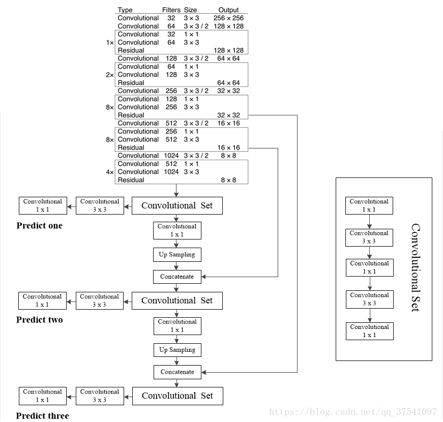
The configuration file here describes the layout of the network, block by block. You can also see the full architecture Darknet-53 in the folloing diagram.

There are 5 types of layers that are used in YOLO:

Convolutional

Shortcut（Residual）: 参数from:-3表示shortcut的output等于倒数第三层的output与前一层output相加

Upsample: YOLO3采用了类似FPN的结构，在三个尺度上进行预测，故要做两次unsample

Route：
When layers attribute has only one value, it outputs the feature maps of the layer indexed by the value. In our example, it is -4, so the layer will output feature map from the 4th layer backwards from the Route layer.

When layers has two values, it returns the concatenated feature maps of the layers indexed by it’s values. In our example it is -1, 61, and the layer will output feature maps from the previous layer (-1) and the 61st layer, concatenated along the depth dimension.

[route]
layers = -4

[route]
layers = -1, 61

YOLO：
The anchors describes 9 anchors, but only the anchors which are indexed by attributes of the mask tag are used.

[yolo]
mask = 0,1,2
anchors = 10,13,  16,30,  33,23,  30,61,  62,45,  59,119,  116,90,  156,198,  373,326
classes=80
num=9
jitter=.3
ignore_thresh = .5
truth_thresh = 1
random=1

Parsing the configuration file

def parse_cfg(cfgfile):
    """
    Takes a configuration file
    
    Returns a list of blocks. Each blocks describes a block in the neural
    network to be built. Block is represented as a dictionary in the list
    
    """

Creating the building blocks

def create_modules(blocks):
    net_info = blocks[0]     #Captures the information about the input and pre-processing    
    module_list = nn.ModuleList()
    prev_filters = 3
    output_filters = []

Our function will return a nn.ModuleList .

prev_filters is used to keep track of number of filters in the layer on which the convolutional layer is being applied.

output_filters is used to store the number of output filters of each block, for route layer need.

1 2	for x in blocks: module = nn.Sequential()

nn.Sequential class is used to sequentially execute a number of nn.Module objects. We use it’s add_module function to string together all layers.

for conv layer and unsample layer:(PyTorch has provided pre-built layers)

#Add the convolutional layer
conv = nn.Conv2d(prev_filters, filters, kernel_size, stride, pad, bias = bias)
module.add_module("conv_{0}".format(index), conv)

#Add the Batch Norm Layer
bn = nn.BatchNorm2d(filters)
module.add_module("batch_norm_{0}".format(index), bn)

#Check the activation. 
#It is either Linear or a Leaky ReLU for YOLO
activn = nn.LeakyReLU(0.1, inplace = True)
module.add_module("leaky_{0}".format(index), activn)

#If it's an upsampling layer
#We use Bilinear2dUpsampling
upsample = nn.Upsample(scale_factor = 2, mode = "bilinear")
module.add_module("upsample_{}".format(index), upsample)

for Route Layer / Shortcut Layers:

shortcut = EmptyLayer()
module.add_module("shortcut_{}".format(index), shortcut)

route = EmptyLayer()
module.add_module("route_{0}".format(index), route)

The empty layer is defined as:

1
2
3

class EmptyLayer(nn.Module):
    def __init__(self):
        super(EmptyLayer, self).__init__()

We use empty layer and perform the concatenation directly in theforward function of the nn.Module object representing darknet.

for yolo layers:

1 2	detection = DetectionLayer(anchors) module.add_module("Detection_{}".format(index), detection)

We define a new layerDetectionLayer that holds the anchors used to detect bounding boxes.

The detection layer is defined as: (the forward function will be proposed later)

class DetectionLayer(nn.Module):
    def __init__(self, anchors):
        super(DetectionLayer, self).__init__()
        self.anchors = anchors

At the end of the loop for each block， we do some bookkeeping.

module_list.append(module)
prev_filters = filters
output_filters.append(filters)
index += 1

At the end of the function create_modules, we return a tuple containing the net_info, and module_list.

2. Implementing the the forward pass of the network

Defining the Network

class Darknet(nn.Module):
    def __init__(self, cfgfile):
        super(Darknet, self).__init__()
        self.blocks = parse_cfg(cfgfile)
        self.net_info, self.module_list = create_modules(self.blocks)

Implementing the forward pass of the network

forward serves two purposes. First, to calculate the output, and second, to transform the output detection feature maps in a way that it can be processed easier

def forward(self, x, CUDA):
    modules = self.blocks[1:]  # the first element is net layer which is no use
    outputs = {}   # We cache the outputs for the route layer
    
    write = 0     #This is explained a bit later
	for i, module in enumerate(modules):        
    	module_type = (module["type"])

Since route and shortcut layers need output maps from previous layers, we cache the output feature maps of every layer in a dict outputs. The keys are the the indices of the layers, and the values are the feature maps.

Convolutional and Upsample Layers

1 2	if module_type == "convolutional" or module_type == "upsample": x = self.module_list[i](x)

Route Layer / Shortcut Layer

elif module_type == "route":
    layers = module["layers"]
    layers = [int(a) for a in layers]

    if (layers[0]) > 0:
        layers[0] = layers[0] - i

    if len(layers) == 1:
        x = outputs[i + (layers[0])]

    else:
        if (layers[1]) > 0:
            layers[1] = layers[1] - i

        map1 = outputs[i + layers[0]]
        map2 = outputs[i + layers[1]]

        x = torch.cat((map1, map2), 1) # concatenate the feature maps along the depth

elif  module_type == "shortcut":
    from_ = int(module["from"])
    x = outputs[i-1] + outputs[i+from_]

In PyTorch, input and output of a convolutional layer has the format B x C x H x W. The depth corresponding the the channel dimension.

YOLO (Detection Layer)

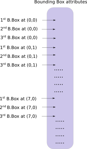
The output of YOLO is a convolutional feature map that contains the bounding box attributes along the depth of the feature map.

There are two problems. First, the attributes bounding boxes predicted by a cell are stacked one by one along each other, this form is very inconvenient for output processing. Second, it would be nice to have to do these operations on a single tensor, rather than three separate tensors.

To remedy these problems, we will introduce the function predict_transform first.

Transforming the output

1	def predict_transform(prediction, inp_dim, anchors, num_classes, CUDA = True):

This function takes an detection feature map and turns it into a 2-D tensor, where each row of the tensor corresponds to attributes of a bounding box, in the following order .

The code to do above transformation is:

batch_size = prediction.size(0)
stride =  inp_dim // prediction.size(2)
grid_size = inp_dim // stride
bbox_attrs = 5 + num_classes
num_anchors = len(anchors)

prediction = prediction.view(batch_size, bbox_attrs*num_anchors, grid_size*grid_size)
prediction = prediction.transpose(1,2).contiguous()
prediction = prediction.view(batch_size, grid_size*grid_size*num_anchors, bbox_attrs)

The dimensions of the anchors are in accordance to the height and width attributes of the net block. These attributes describe the dimensions of the input image, which is larger (by a factor of stride) than the detection map. Therefore, we must divide the anchors by the stride of the detection feature map.

1	anchors = [(a[0]/stride, a[1]/stride) for a in anchors]

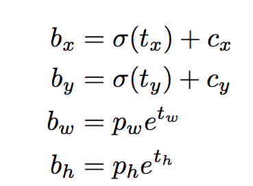
Now, we need to transform our output according to the equations

First, sigmoid the x,y coordinates and the objectness score.

#Sigmoid the  centre_X, centre_Y. and object confidencce
prediction[:,:,0] = torch.sigmoid(prediction[:,:,0])
prediction[:,:,1] = torch.sigmoid(prediction[:,:,1])
prediction[:,:,4] = torch.sigmoid(prediction[:,:,4])

Add the grid offsets to the center cordinates prediction.

#Add the center offsets
grid = np.arange(grid_size)
a,b = np.meshgrid(grid, grid)

x_offset = torch.FloatTensor(a).view(-1,1)
y_offset = torch.FloatTensor(b).view(-1,1)

if CUDA:
    x_offset = x_offset.cuda()
    y_offset = y_offset.cuda()

x_y_offset = torch.cat((x_offset, y_offset), 1).repeat(1,num_anchors).view(-1,2).unsqueeze(0)

prediction[:,:,:2] += x_y_offset

Apply the anchors to the dimensions of the bounding box.

#log space transform height and the width
anchors = torch.FloatTensor(anchors)

if CUDA:
    anchors = anchors.cuda()

anchors = anchors.repeat(grid_size*grid_size, 1).unsqueeze(0)
prediction[:,:,2:4] = torch.exp(prediction[:,:,2:4])*anchors

Apply sigmoid activation to the the class scores.

1	prediction[:,:,5: 5 + num_classes] = torch.sigmoid((prediction[:,:, 5 : 5 + num_classes]))

The last thing we want to do here, is to resize the detections map to the size of the input image. The bounding box attributes here are sized according to the feature map (say, 13 x 13). If the input image was 416 x 416, we multiply the attributes by 32, or the stride variable.

1
2
3

prediction[:,:,:4] *= stride

return prediction

Detection Layer Revisited

elif module_type == 'yolo':        
    anchors = self.module_list[i][0].anchors
    #Get the input dimensions
    inp_dim = int (self.net_info["height"])

    #Get the number of classes
    num_classes = int (module["classes"])

    #Transform 
    x = x.data
    x = predict_transform(x, inp_dim, anchors, num_classes, CUDA)
    if not write:              #if no collector has been intialised. 
        detections = x
        write = 1

    else:       
        detections = torch.cat((detections, x), 1)

outputs[i] = x

rturn detections

3. Confidence Thresholding and Non-maximum Suppression

To be precise, our output is a tensor of shape B x 10647 x 85. B is the number of images in a batch, 10647 is the number of bounding boxes predicted per image, and 85 is the number of bounding box attributes.

However, we must subject our output to objectness score thresholding and Non-maximal suppression, to obtain what we will call in the rest of this post as thetrue detections. To do that, we will create a function called write_results.

1	def write_results(prediction, confidence, num_classes, nms_conf = 0.4):

Object Confidence Thresholding

1 2	conf_mask = (prediction[:,:,4] > confidence).float().unsqueeze(2) prediction = prediction*conf_mask

Performing Non-maximum Suppression

Transform the (center x, center y, height, width) attributes of our boxes, to (top-left corner x, top-left corner y, right-bottom corner x, right-bottom corner y).

box_corner = prediction.new(prediction.shape)
box_corner[:,:,0] = (prediction[:,:,0] - prediction[:,:,2]/2)
box_corner[:,:,1] = (prediction[:,:,1] - prediction[:,:,3]/2)
box_corner[:,:,2] = (prediction[:,:,0] + prediction[:,:,2]/2) 
box_corner[:,:,3] = (prediction[:,:,1] + prediction[:,:,3]/2)
prediction[:,:,:4] = box_corner[:,:,:4]

Confidence thresholding and NMS has to be done for one image at once. This means, we must loop over the first dimension of prediction.

batch_size = prediction.size(0)

write = False

for ind in range(batch_size):
    image_pred = prediction[ind]          #image Tensor
       #confidence threshholding 
       #NMS

Notice each bounding box row has 85 attributes, out of which 80 are the class scores. At this point, we’re only concerned with the class score having the maximum value. So, we remove the 80 class scores from each row, and instead add the index of the class having the maximum values, as well the class score of that class.

max_conf, max_conf_score = torch.max(image_pred[:,5:5+ num_classes], 1)
max_conf = max_conf.float().unsqueeze(1)
max_conf_score = max_conf_score.float().unsqueeze(1)
seq = (image_pred[:,:5], max_conf, max_conf_score)
image_pred = torch.cat(seq, 1)

Get rid of the bounding box rows having a object confidence less than the threshold.

non_zero_ind =  (torch.nonzero(image_pred[:,4]))
try:
    image_pred_ = image_pred[non_zero_ind.squeeze(),:].view(-1,7)
except:
    continue

#For PyTorch 0.4 compatibility
#Since the above code with not raise exception for no detection 
#as scalars are supported in PyTorch 0.4
if image_pred_.shape[0] == 0:
    continue

The try-except block is there to handle situations where we get no detections. In that case, we use continue to skip the rest of the loop body for this image.

Now, let’s get the classes detected in a an image.

1 2	#Get the various classes detected in the image img_classes = unique(image_pred_[:,-1]) # -1 index holds the class index

Since there can be multiple true detections of the same class, we use a function called unique to get classes present in any given image.

def unique(tensor):
    tensor_np = tensor.cpu().numpy()
    unique_np = np.unique(tensor_np)
    unique_tensor = torch.from_numpy(unique_np)
    
    tensor_res = tensor.new(unique_tensor.shape)
    tensor_res.copy_(unique_tensor)
    return tensor_res

Then, we perform NMS classwise.

1 2	for cls in img_classes: #perform NMS

Once we are inside the loop, the first thing we do is extract the detections of a particular class (denoted by variable cls).

#get the detections with one particular class
cls_mask = image_pred_*(image_pred_[:,-1] == cls).float().unsqueeze(1)
class_mask_ind = torch.nonzero(cls_mask[:,-2]).squeeze()
image_pred_class = image_pred_[class_mask_ind].view(-1,7)

#sort the detections such that the entry with the maximum objectness confidence is at the top
conf_sort_index = torch.sort(image_pred_class[:,4], descending = True )[1]
image_pred_class = image_pred_class[conf_sort_index]
idx = image_pred_class.size(0)   #Number of detections

Now, we perform NMS.

for i in range(idx):
    #Get the IOUs of all boxes that come after the one we are looking at 
    #in the loop
    try:
        ious = bbox_iou(image_pred_class[i].unsqueeze(0), image_pred_class[i+1:])
    except ValueError:
        break

    except IndexError:
        break

    #Zero out all the detections that have IoU > treshhold
    iou_mask = (ious < nms_conf).float().unsqueeze(1)
    image_pred_class[i+1:] *= iou_mask       

    #Remove the non-zero entries
    non_zero_ind = torch.nonzero(image_pred_class[:,4]).squeeze()
    image_pred_class = image_pred_class[non_zero_ind].view(-1,7)

Here, we use a function bbox_iou. The first input is the bounding box row that is indexed by the the variable i in the loop.
Second input is a tensor of multiple rows of bounding boxes. The output of the function bbox_iou is a tensor containing IoUs of the bounding box represented by the first input with each of the bounding boxes present in the second input.
If we have two bounding boxes of the same class having an IoU larger than a threshold, then the one with lower class confidence is eliminated.

Also notice, we have put the line of code to compute the ious in a try-catch block. This is because the loop is designed to run idx iterations. However, as we proceed with the loop, a number of bounding boxes may be removed from image_pred_class. This means, we cannot have idx iterations in most instances. Hence, we might try to index a value that is out of bounds (IndexError), or the slice image_pred_class[i+1:] may return an empty tensor, assigning which triggers a ValueError. At that point, we can ascertain that NMS can remove no further bounding boxes, and we break out of the loop.

Calculating the IoU

def bbox_iou(box1, box2):
    """
    Returns the IoU of two bounding boxes 
    """
    #Get the coordinates of bounding boxes
    b1_x1, b1_y1, b1_x2, b1_y2 = box1[:,0], box1[:,1], box1[:,2], box1[:,3]
    b2_x1, b2_y1, b2_x2, b2_y2 = box2[:,0], box2[:,1], box2[:,2], box2[:,3]
    
    #get the corrdinates of the intersection rectangle
    inter_rect_x1 =  torch.max(b1_x1, b2_x1)
    inter_rect_y1 =  torch.max(b1_y1, b2_y1)
    inter_rect_x2 =  torch.min(b1_x2, b2_x2)
    inter_rect_y2 =  torch.min(b1_y2, b2_y2)
    
    #Intersection area
    inter_area = torch.clamp(inter_rect_x2 - inter_rect_x1 + 1, min=0) * torch.clamp(inter_rect_y2 - inter_rect_y1 + 1, min=0)
 
    #Union Area
    b1_area = (b1_x2 - b1_x1 + 1)*(b1_y2 - b1_y1 + 1)
    b2_area = (b2_x2 - b2_x1 + 1)*(b2_y2 - b2_y1 + 1)
    
    iou = inter_area / (b1_area + b2_area - inter_area)
    
    return iou

Writing the predictions

The function write_results outputs a tensor of shape D x 8. Here D is the true detections in all of images, each represented by a row. Each detections has 8 attributes, namely, index of the image in the batch to which the detection belongs to, 4 corner coordinates, objectness score, the score of class with maximum confidence, and the index of that class.

batch_ind = image_pred_class.new(image_pred_class.size(0), 1).fill_(ind)      
#Repeat the batch_id for as many detections of the class cls in the image
seq = batch_ind, image_pred_class

if not write:
    output = torch.cat(seq,1)
    write = True
else:
    out = torch.cat(seq,1)
    output = torch.cat((output,out))

4. Designing the input and the output pipelines

Loading the Network

Load the class file.

1 2	num_classes = 80 #For COCO classes = load_classes("data/coco.names")

def load_classes(namesfile):
    fp = open(namesfile, "r")
    names = fp.read().split("\n")[:-1]
    return names

Initialize the network and load weights.

#Set up the neural network
print("Loading network.....")
model = Darknet(args.cfgfile)
model.load_weights(args.weightsfile)
print("Network successfully loaded")

model.net_info["height"] = args.reso
inp_dim = int(model.net_info["height"])
assert inp_dim % 32 == 0 
assert inp_dim > 32

#If there's a GPU availible, put the model on GPU
if CUDA:
    model.cuda()

#Set the model in evaluation mode
model.eval()

Read the Input images

read_dir = time.time()
#Detection phase
try:
    imlist = [osp.join(osp.realpath('.'), images, img) for img in os.listdir(images)]
except NotADirectoryError:
    imlist = []
    imlist.append(osp.join(osp.realpath('.'), images))
except FileNotFoundError:
    print ("No file or directory with the name {}".format(images))
    exit()

use OpenCV to load the images.

1 2	load_batch = time.time() loaded_ims = [cv2.imread(x) for x in imlist]

Write the function letterbox_image to resizes our image, keeping the aspect ratio consistent, and padding the left out areas with the color (128,128,128).

def letterbox_image(img, inp_dim):
    '''resize image with unchanged aspect ratio using padding'''
    img_w, img_h = img.shape[1], img.shape[0]
    w, h = inp_dim
    new_w = int(img_w * min(w/img_w, h/img_h))
    new_h = int(img_h * min(w/img_w, h/img_h))
    resized_image = cv2.resize(img, (new_w,new_h), interpolation = cv2.INTER_CUBIC)
    
    canvas = np.full((inp_dim[1], inp_dim[0], 3), 128)

    canvas[(h-new_h)//2:(h-new_h)//2 + new_h,(w-new_w)//2:(w-new_w)//2 + new_w,  :] = resized_image
    
    return canvas

Write the function prep_image to takes a OpenCV images and converts it to PyTorch’s input format.

def prep_image(img, inp_dim):
    """
    Prepare image for inputting to the neural network. 
    
    Returns a Variable 
    """

    img = cv2.resize(img, (inp_dim, inp_dim))
    img = img[:,:,::-1].transpose((2,0,1)).copy()
    img = torch.from_numpy(img).float().div(255.0).unsqueeze(0)
    return img