Using a series of low dynamic range images at different exposure
Generally, this problem can be broken down into two stages: 1) aligning the input LDR images and 2) merging the aligned images into an HDR image.
This method produces spectacular images for tripod mounted cameras and static scenes, but generates results with ghosting artifacts when the scene is dynamic or the camera is hand-held.
Deep High Dynamic Range Imaging of Dynamic Scenes - SIGGRAPH2017
-the artifacts of the alignment can be significantly reduced during merging
-Preprocessing the Input LDR Images:
If the LDR images are not in the RAW format, we first linearize them using the camera response function (CRF), then apply gamma correction (γ = 2.2). The gamma correction basically maps the images into a domain that is closer to what we perceive with our eyes.
-Alignment:
Produce aligned images by registering the images with low (Z1) and high (Z3) exposures to the reference image Z2 using tranditional method. (optical flow)
-HDR Merge:
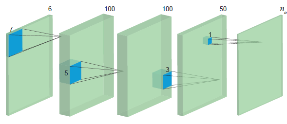
1)Model: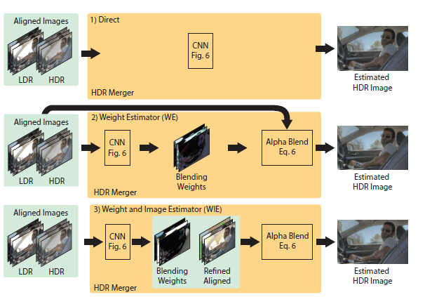
2)Loss Function:
Since HDR images are usually displayed after tonemapping, we propose to compute our loss function between the tonemapped estimated and ground truth HDR images. We propose to use μ-law, a commonly-used range compressor in audio processing, which is differentiable.
we train the learning system by minimizing the L2 distance of the tonemapped estimated and
ground truth HDR images defined as:
Deep High Dynamic Range Imaging with Large Foreground Motions - ECCV2018
-CNNs have been demonstrated to have the ability to learn misalignment and hallucinate missing details
-Three advantage: 1) trained end-to-end without optical flow alignment. 2)can hallucinate plausible details that are totally missing or their presence is extremely weak in all LDR inputs. 3) the same framework can be easily extended to more LDR inputs, and possibly with any specified reference image.
-Network Architecture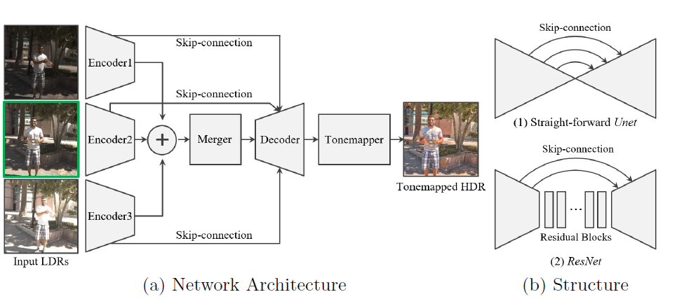
We separate the first two layers as encoders for each exposure inputs. After extracting the features, the network learns to merge them, mostly in the middle layers, and to decode them into an HDR output, mostly in the last few layers.
-Processing Pipeline and Loss Function
Given a stack of LDR images, if they are not in RAW format, we first linearize the images using the estimated inverse of Camera Response Function (CRF), which is often referred to as radiometric calibration. We then apply gamma correction to produce the input to our system.
We first map LDRs to H = {H1;H2;H3} in the HDR domain, using simple gamma encoding:
where ti is the exposure time of image Ii. We then concatenate I and H channel-wise into a 6-channel input and feed it directly to the network. The LDRs facilitate the detection of misalignments and saturation, while the exposure-adjusted HDRs improve the robustness of the network across LDRs with various exposure levels.
Tonemapping function and loss function are the same as the previous paper.
-Data Preparation
First align the background using simple homography transformation by homography transformation. Without it, we found that our network tends to produce blurry edges where background is largely misaligned.
Crop the images into 256x256 patches with a stride of 64. To keep the training focused on foreground motions, we detect large motion patches by thresholding the structural similarity between different exposure shots, and replicate these patches in the training set.
Using single low dynamic range image
One intrinsic limitation of this approach is the total reliance on one single input LDR image, which often fails in highly contrastive scenes due to large-scale saturation.
HDR image reconstruction from a single exposure using deep CNNs - 1710
-Estimating missing information in bright image parts, such as highlights, lost due to saturation of the camera sensor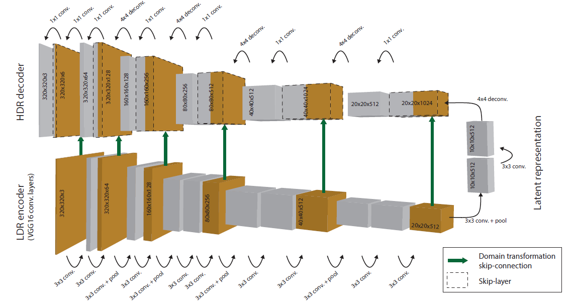
ExpandNet: A Deep Convolutional Neural Network for High Dynamic Range Expansion from Low Dynamic Range Content - EUROGRAPHICS 2018
-Designed to avoid upsampling of downsampled features, in an attempt to reduce blocking and/or haloing artefacts that may arise from more straightforward approaches.
-It is argued that upsampling, especially the frequently used deconvolutional layers, cause checkerboard artefacts. Furthermore, upsampling may cause unwanted information bleeding in areas where context is missing, for example large overexposed areas.
-The local branch handling local detail, the dilation branch for medium level detail, and a global branch accounting for higher level image-wide features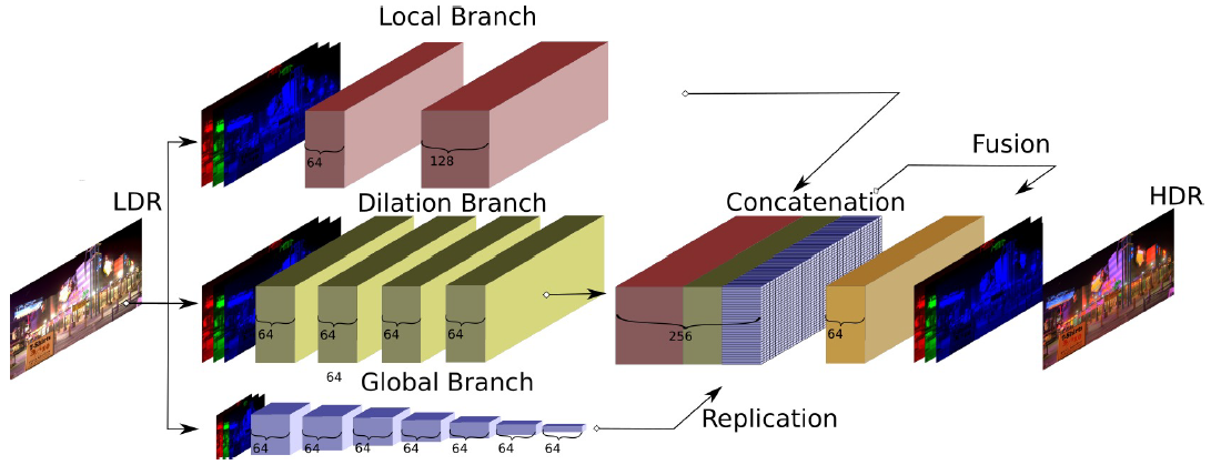
-Loss Function
The L1 distance is chosen for this problem since the more frequently used L2 distance was found to cause blurry results for images. An additional cosine similarity term is added to ensure color correctness of the RGB vectors of each pixel.
Cosine similarity measures how close two vectors are by comparing the angle between them, not taking magnitude into account. For the context of this work, it ensures that each pixel points in the same direction of the three dimensional RGB space. It provides improved color stability, especially for low luminance values, which are frequent in HDR images, since slight variations in any of the RGB components of these low values do not contribute much to the L1 loss, but they may however cause noticeable color shifts.
Dataset
proposed by Kalantari(Deep High Dynamic Range Imaging of Dynamic Scenes):
To generate the ground truth HDR image, we capture a static set by asking a subject to stay still and taking three images with different exposures on a tripod.
Next, we capture a dynamic set to use as our input by asking the subject to move and taking three bracketed exposure images either by holding the camera (to simulate camera motion) or on a tripod.
Capture all the images in RAW format with a resolution of 5760 × 3840 and using a Canon EOS-5D Mark III camera. Downsample all the images (including the dynamic set) to the resolution of 1500 × 1000.
Use color channel swapping and geometric transformation (rotating 90 degrees and flipping) with 6 and 8 different combinations, respectively. This process produces a total of 48 different combinations of data augmentation, from which we randomly choose 10 combinations to augment each training scene. Our data augmentation process increases the number of training scenes from 74 to 740.
Finally, since training on full images is slow, we break down the training images into overlapping patches of size 40 × 40 with a stride of 20. This process produces a set of training patches consisting of the aligned patches in the LDR and HDR domains as well as their corresponding ground truth HDR patches. We then select the training patches where more than 50 percent of their reference patch is under/over-exposed, which results in around 1,000,000 selected patches. This selection is performed to put the main focus of the networks on the challenging regions.
Described in DeepHDR
The dataset was split into 74 training examples and 15 testing examples. crop the images into 256x256 patches with a stride of 64, which produces around 19000 patches. We then perform data augmentation (flipping and rotation), further increasing the training data by 8 times.
In fact, a large portion of these patches contain only background regions, and exhibit little foreground motions. To keep the training focused on foreground motions, we detect large motion patches by thresholding the structural similarity
between different exposure shots, and replicate these patches in the training set.
ExpandNet
Results
Sen: Robust Patch-Based HDR Reconstruction of Dynamic Scenes. ACM TOG 31(6), 203:1-203:11 (2012)
Hu: HDR Deghosting: How to deal with Saturation? In: IEEE CVPR (2013)
Kalantari: Deep High Dynamic Range Imaging of Dynamic Scenes. ACM TOG 36(4) (2017)
HDRCNN: HDR image reconstruction from a single exposure using deep cnns. ACM TOG 36(6) (2017)
Ours: Deep High Dynamic Range Imaging with Large Foreground Motions
Running Time
PC with i7-4790K (4.0GHz) and 32GB RAM, 3 LDR images of size 896x1408 as input.

When run with GPU (Titan X Pascal), our Unet and ResNet take 0.225s and 0.239s respectively.
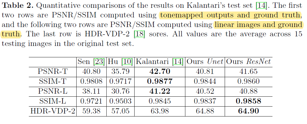
Quantitative Comparison
